 GBR
GBR Included in collection: Microeconomics
Consumer Choice Theory Lecture
Chapter Summary
Welcome to the next lesson of this module where we will cover the topic of consumer choice theory.
The following chapter will discuss consumer choice, where we will consider why we make the consumption choices we do. The chapter will consider sections on utility maximisation, budget constraints and composite goods. By the end of the chapter you should have met the following learning objectives:
- Understand consumer preferences and understand how you would approach the analysis of their choice with the use of indifference curves.
- Explain the concept of the budget constraint, and be able to explain why prices must be paid for various goods.
- Understand how the ‘market basket’ chosen by a consumer is determined by (1) the consumer’s preferences and (2) the budget constraints imposed on the consumer by income and the prices that must be paid for various goods.
- Determine how changes in income will affect the consumption choices of the consumer.
- Understand if consumers are selfish, or if there is a hint of altruism[1] involved.
- Understand the concept of utility, and relate this back to the indifference curves.
Need Help With Your Economics Essay?
If you need assistance with writing a economics essay, our professional essay writing service can provide valuable assistance.
See how our Essay Writing Service can help today!
1.0 Consumer Choice
The following chapter will discuss consumer choice, considering theory behind utility maximisation, opportunity costs and consumer preferences. The theory of consumer choice is focused in microeconomics, relating to preferences for consumer expenditure, which in turn impacts on consumer demand curves. For instance, one use of consumer theory is to showcase why the demand curve for many goods slopes downward. However, moving on from these basic principles, consumer choice, and so consumer behaviour have far greater implications. In business, consumer behaviour theories are used by firms to consider why a consumer purchasing a car may place a greater value on safety over fuel mileage; it could be used by some businesses when it comes to determining their strategy. For example, Ryanair dominates the low-cost airline market with a focus on price, however other airlines, be it British Airways continue to offer the same product but at a higher price, using consumer choice theories to understand the added value which they can generate for their products from added services.
Economists also have extended consumer choice theory to individuals’ decisions concerning labour supply, saving and investment, charitable contributions, voting, and even marriage, showing how the theories mentioned in this chapter can be applied. When it comes to consumer expenditure, it must be remembered that the consumer in question will always be constrained in expenditure by their earnings, which in turn will create a ‘cost’ to their spending decisions.
Observations will tell us that consumer choices differ widely, be it between countries/ demographics, or just between one consumer and another. For instance, some may prefer chicken, while others may prefer pork etc. Taking this into account, there is such diversity in choices which may present a challenge for economists. However, to overcome these challenges, economists will base their analysis on general propositions; making three general assumptions. The first assumption is that consumer preferences are complete, meaning that they can rank all market baskets in the order of their choice. So, considering Coca Cola and Pepsi, a consumer could either say that they prefer Coca Cola to Pepsi, Pepsi to Coca Cola, or are indifferent between the two. When the word indifferent is used, it means that the consumer has no preference, they are both equally satisfactory. However, what must be mentioned here is that while the consumer may be indifferent to these two items, the preference is relative of the products, rather than the price; this can also be said for all preference rankings. So, it is plausible to consider that a consumer may prefer a BMW to a Ford; however, may still end up buying the Ford given the relative prices of both products coupled with their own income.
The second assumption would be that preferences are transitive. This can be explained simple with the following example. Assume that a consumer prefers product A to B, and product B to C; then logically, the consumer must prefer product A to C.
Finally, the third assumption is that the consumer will prefer more goods to less. So, in the case of a holiday, the consumer will prefer two holidays to one. This assumption will later lead into a discussion on utility maximisation. However, the third assumption has always been up for discussion, with some arguing that this idea that a consumer prefers more goes against businesses which may seek to sell luxury products. For instance, a luxury holiday business may base its business model on selling high-cost holidays under the assumption that the consumer may enjoy one holiday to The Maldives over two holidays to Benidorm. Furthermore, there is also this idea of economic ‘bads’, which are classed as goods which consumers prefer less off than more; for instance, pollution. An economic “good” be the opposite, and is a good which more is better than less; in effect, it is a desirable commodity; for instance, chocolate.
So, moving on from these assumptions we can now consider ‘Indifference Curves’ (pictured below). These curves can also be called Consumer Preference Graphs as the chart will plot all the combinations of the two goods which offer the consumer the same utility. In this case, they would be indifferent when it comes to choosing anyone of them given that the utility received is the same.
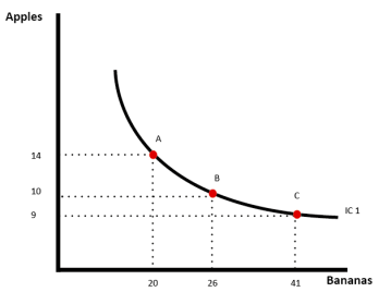
Figure 1 - Indifference Curve for Apples vs. Banana’s
From analysing these curves, we can note several assumptions. The first is that the indifference curve must slope downward if the consumer views these goods as desirable. The main reason behind this is that all baskets of goods which are equally satisfactory to the consumer must contain less of one good, replaced in turn by more of another; creating this downward slope. The second assumption is that a consumer will always prefer a basket of goods towards the Northeast of the slope given the expectation of higher utility. On other hand, any basket of goods which lies below the indifference curve will be viewed as less desirable; we should always remember that a consumer will look to maximise their utility given the resources they have; i.e. income. However, in some circumstances it may be noted that the indifference curve is not always a curve as shown above. For instance, consider the example of two goods which are perfect complements; i.e. printer and ink cartridges. In this case, a consumer who demands a printer will also demand ink cartridges, and so there is no substitution.
Taking the above, we have analysed just one indifference curve, however multiple curves could be added to showcase an indifference map (shown below). So, every basket available on the higher indifference curves will be preferred to that on the lower curves, however as we have mentioned there could be some constraints to a consumer moving into the higher curves; i.e. their disposable income.
The indifference map does good at providing a ranking to baskets (shown below), however as you may have spotted, it provides little in the way of information into by how much a consumer may prefer one basket to another. Now that we have shown an indifference map it is also important to mentioned the third assumption behind these curve; that two indifference curves should not intersect.
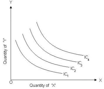
Figure 2 - Visualisation of an Indifference Map.
1.1 Curvature of the Indifference Curve
The three features of indifference curves have been mentioned: they slope downward, higher curves are preferred to lower ones, and they cannot intersect. Convexity can be seen as a fourth feature of indifference curves. The convexity brings into consideration the marginal rate of substitution, otherwise abbreviated as MRS. So, a consumers MRS between chocolate, and apples is the maximum amount of chocolate that the consumer is willing to give up to obtain an additional apple. Essentially, it can be viewed as the willingness to trade one good for another. The complexity in this comes from that fact that the rate may differ depending on the actual quantity of the good already held. For instance, if a consumer has 10 chocolate bars, they may be more willing to trade a chocolate bar for an apple then say compared to their willingness to trade if they only had 2 chocolate bars. There is also a question over how much of one good must be traded for another. For example, it may not be as simple as 1 chocolate bar for one apple; maybe its 2 chocolate bars for 1 apple.
We consider the diminishing MRS along the indifference curve, with the key word here being diminishing given the expectation that as the quantity of a good decreases, they are less willing to trade. This can be seen in the figure below:

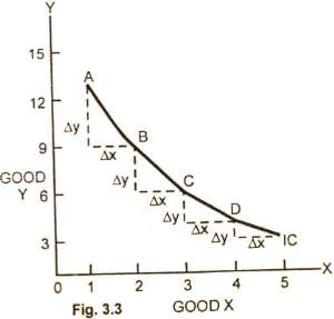
Figure 3 - A visualisation of Marginal Rate of Substitution. As the consumer loses more of Good Y, they become more reluctant to give up further units for Good X.
So, when the consumer has 20 chocolate and 0 apples, they may be willing to give a maximum of 3 chocolate in exchange for 1 apple, see table below. However, as their quantity of chocolate diminishes they place a higher value on it, leading to the maximum they may be willing to trade falling to 1 chocolate for 2 apples etc., and then none.
|
Combination |
Chocolates |
Apples |
MRS for Goods |
|
1 |
20 |
0 |
-- |
|
2 |
14 |
2 |
3 : 1 |
|
3 |
10 |
4 |
2 : 1 |
|
4 |
9 |
6 |
1 : 2 |
1.2 Choice - Utility Maximisation under Budget Constraint
When consumer choice is considered, the idea of consumer utility is also considered. Utility can be imagined as the satisfaction/ enjoyment that a consumer may receive from consuming a certain product. This leads to a decision as the consumer will look to maximise their utility based on purchasing a number of goods which allow them to reach the highest possible total utility. However, as mentioned before, the consumer will be constrained in their spending by their income; known as their budget constraint.
The law of ‘Diminishing Returns’ must also be considered here given that it could be expected that as a consumer demands more of a particular good; the utility received from that good decreases. This is mentioned above in our discussion on MRS. However, what needs to be added here is the idea of the budget constraint, and how this impacts on utility.
Example
Suppose that you have a total of £10 to spend on your lunch. You make you way into a food outlet where you can buy the goods shown below:
|
Sandwich |
£4.00 |
|
Chocolate |
£2.00 |
|
Pastry |
£3.00 |
|
Drink |
£2.00 |
Buying the first sandwich may give the consumer a high level of satisfaction, alleviating hunger. However, if the consumer then went to buy another sandwich, the actual satisfaction from the second may be lower than the first; for instance, the food could be repetitive, too much etc., leading to less enjoyment. Instead, the consumer may get more enjoyment from purchasing a drink/ pastry. Ultimately, the consumer will look to choose the combination of goods which (1) meets the budget constraint, and (2) offers the greatest utility. This example will be touched upon later in the chapter when opportunity cost is discussed.
So what is being discussed in the example above is that as a consumer demands more of one good, the marginal utility, and so the utility from one more begins to fall. However, the consumer may still continue to demand more as long as the marginal utility received is greater than the price being paid for by the good. With this in mind, there is some link between the utility of the good and the price elasticity of the good. To provide a definition, the price elasticity of the good will showcase how customers will react with demand given a change in the price. So, for instance, how demand for a certain good will be impacted by an increase in the price?
To determine the price elasticity of a good the first step will be to consider the change in price. So, if the price of the good increased from £20 to £22, then the increase is 2/20 = 0.1, or 10%. Secondly, consider the change in demand, so if the quantity demanded fell to 87 from 100, then 13/100 = -0.13 or 13%. Therefore, to calculate the price elasticity of demand we consider the change in quantity, over the change in price, in this case being (-)13/ 10 = -1.3. A result of (-)1.3 would suggest that the elasticity is elastic, and that a higher price will lead to a fall in demand, so the effect is negative. When it comes to determining the elasticity, a results below 1 would suggest that the good is inelastic given that the change in demand is less than the change in price. On the other hand, a result above 1 would suggest elastic demand, being that the demand changes by more than the price. These generally hold, however other researchers have put forward other types of goods, i.e. Veblen Goods. Veblen goods are goods where an increase in price actually leads to an increase in demand, and is usually seen in the luxury sector, whereby a higher price may be a sign of exclusivity, attracting people to demand more of that good.
However, when talking about price elasticity, other factors must also be brought in, including substitution and alternatives. To showcase this, consider two goods, chocolate and petrol. Petrol may be considered as an inelastic good given its need in the economy, be it for industrial processes, or for consumers to fuel their vehicles. Given that consumers may have certain commitments which require petrol such as travelling to work, there is the idea that if prices for petrol did increase, the consumer would have to bear the price increase and maintain demand to continue life as usual. This would be seen in the short-term, however, when we move into the long-term, demand could fall as customers seek alternatives; for instance, public transport, or by purchasing a vehicle which is more fuel efficient.
1.2.1 Changes in a Budget Constraint
When we talk about a budget constraint we consider a Linear function as shown below, with the consumer able to purchase any bundle of good on the line (shown below). In this example, we can see that the consumer can buy any bundle of goods behind the line, denoted as being feasible:
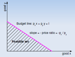
Figure 4 - Linear Budget Constraint.
Although, there are some examples which can affect this linear position. For instance, consider an example whereby the consumer can receive a discount on the price of the good for bulk buying, which in turn would reduce the cost per unit if a certain level is purchased (shown below). Ultimately, the line is no longer linear.
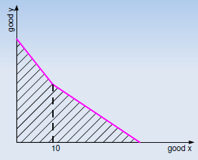
Figure 5 - Budget Constraint with quantity discounts applied.
We can also consider other situations which may affect a consumer in their daily life’s. For instance, some goods may have quantity rationing on, so a consumer may only be able to buy 6 units of a good at a specific price. There may also be goods whereby the quantity consumed is restricted given social norms; for instance, a consumer may only eat so much chocolate to remain healthy, or only drink so many units of alcohol given national recommendations etc.
1.3 Consumer Equilibrium
Taking the example above, the consumer will thus look to maximise their utility given their current budget constraint, which in turn will create an optimal basket of goods, shown below in the diagram:
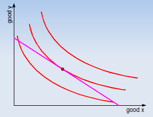
Figure 6 - The optimal basket of goods given the budget constraint.
The point at which the budget line and indifference curve intersect is the optimal point which maximises the consumer utility given their constraints. In this equilibrium, it could be mentioned that the MRS would thus equal the price ratio, denoted as MRSyx = px/ py.
Continuing from the example above, consumer equilibrium could be seen to occur when the marginal utility of the good equals the price which is being paid for the good. Beyond this point, whereby the utility falls lower, the consumer may look to reduce their demand, or substitute their demand for another good.
Although, it must be mentioned that this may depend on the good in question. For instance, if the price of apples increased, then a consumer may look to reduce their demand, potentially substituting apples for pears to maintain total utility. However, other goods, such as petrol may exert a different effect. In terms of petrol, and increase in the price may do little to consumer demand given that petrol for some consumers may be an essential good, needed to get from point A to B.
However, when there is a potential substitute, then the marginal rate of substitution can be considered, which can be seen in the following equation:

1.4 Opportunity Cost
When it comes to discussing utility, there is an element of opportunity cost to be considered. For instance, with a constrained budget, the consumer must make choices based on their own needs. Considering the lunch example once again, the opportunity cost there was that by buying a pastry and gaining the utility, the consumer was foregoing the utility which could be gained from spending that money on chocolate, or drink. Opportunity cost can be noted in many real world examples. For instance, if the price of petrol increased, then the consumer may choose to cut spending on entertainment to maintain their demand for petrol, however the opportunity cost involved here is the lost utility from not going to the cinema, or bowling etc. Ultimately, it is defined as the value of the forgone activity/ or alternative when another activity/ good is chosen. It can be visualised with the following equation:
Opportunity Cost = Return of Most Lucrative Option - Return of Chosen Option
However, what must be mentioned when it comes to opportunity cost is that such is a forward looking equation, and so in this case the ‘Return’ may be hard to accurately calculate as it is not known. For instance, considering the example above with petrol/ entertainment; the consumer may not know how much utility (return) they would gain from the entertainment until they have actually done it.
1.5 Pareto Efficiency
Leading on from opportunity cost, Pareto Efficiency can be considered. The basic assumption under Pareto efficiency is that it is impossible to make one person better off without making someone else worse off. So, when it comes to allocating resources in an economy, helping one person improve their own preference criterion will lead to another being worse off. This could be considered in regards to a business who has a set budget to meet. If the business decided to offer a wage increase to a specific department, costs may need to be cut in another department to ensure that the budget is maintained.
Usually, the Pareto Efficiency will be considered alongside the Production Possibility Frontier, hereafter PPF (see below), a graph which considers the combination of production available for two goods:
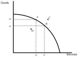
Figure 7 - Visual representation of the Production Possibility Frontier.
In the case above, the economy cannot increase the production of one good without decreasing production of the other; similar to what has been mentioned above when it comes to consumer choice and their budget constraint. However, what can also be mentioned in this case is that there is the potential to expand the PPF, in this case through improvements in productivity, or an expansion of the production capacity, and so the economy.
1.6 The Composite-Good Convention
In all the discussions above, we have noted models which feature two goods. However, as most of us will know from being consumers ourselves, there are more than two goods to consider. Although, when it comes to graphing such, it becomes difficult to draw an indifference curve with many, many goods. So, to overcome this, there is the idea of a composite good, which is defined as several goods which are treated as the same. For instance, we may consider the outlay on clothing vs. all other goods, essentially grouping all other goods into a composite. If we have a budget of £100, and spend £20 on clothing, then the idea is that there is a further £80 which can be spent on all other goods.
However, the main issue here is that denoting all other goods into a composite can be difficult given the many types of goods to consider. Above we have already talked about how some goods could be elastic and how some could be inelastic. Added to this is the concept between normal goods and inferior goods, which then brings in the concept of income. For instance, if the consumer’s income rose, the idea with a normal good would be that consumption increases; so, the consumer will consume more. However, there is also the concept of inferior goods; being a good which may see its consumption fall as income rises, with the consumer substituting for another. To provide an example, consider a consumer in China who currently cannot afford meat so denotes all their income to rice. However, as their income rises, they can now afford better food in a sense, and so increase their consumption of meat at the expenses of rice. In this case, rice is the inferior good.
1.7 Edgeworth Box
When it comes to discussing the behaviour of markets in economics, the traditional model used is that of supply/ demand. This can also be considered in regards to consumer choice, with the demand for a product from a consumer potentially falling as the price goes higher. This has been discussed above when utility was considered, with a higher price potentially deterring some consumers from buying the product given the utility it would provide them; they may look to buy a cheaper product which would help them maximise their utility under the constraint of their budget.
Ultimately, equilibrium will be reached when supply/ demand meet. From here, General Equilibrium Analysis is seen as an extension of the theory, noting how supply/ demand conditions will interact in several markets to determine the price of a number of goods. From this, the Edgeworth Box can now be explained. The Edgeworth Box can be seen as analysis which considers the interaction of two individuals trading in two different commodities, which the image below providing a visualisation of the theory:
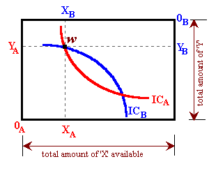
Figure 8 - Visualisation of The Edgeworth Box.
In the example shown above, the lower-left corner represents consumer A, while the top-right represents consumer B. In the middle are the indifference curves, which represents the combinations of the two goods where the consumer is indifferent; and so the consumer has no preference for the bundle of goods they will receive. As shown in the image, point ‘W’ represents what could be considered as a starting equilibrium as both indifference curves meet. Rather than introduce budget lines into the graph, the theory considers the concept of initial endowments (or income), again seen by point ‘W’.
1.8 Are Consumers Selfish
Taking in all the theory above, the main question to ask now could be whether people would be classed as selfish. Some may comment that of course people are selfish as the underling theory would suggest that a consumer will seek to maximise their own utility based on their budget. Ultimately, they only care for their own utility. However, the economic theory is vague in this respect given that the models above do not specify which goods/ services a consumer would see as desirable. For instance, we can consider that some individuals will seek to give more to charity, or donate their time to a ‘good cause’ as opposed to working and increasing their income. Essentially, while the person may still get a level of utility from this, the actual good would not be classed as selfish given that it is helping someone else. The consumer is viewing such as an economic good.
1.9 Issues to Mention - Consumer Theory
As we have touched upon throughout the piece, while consumer choice theory is useful for businesses to understand the behaviour of their consumers, there are several issues. For instance, we considered above that an issue with indifference curves is that they only consider two goods; in reality, consumers have multiple goods to consider. While there is the potential to use a composite good to group many of these together, it does not completely solve the issue. Furthermore, there is also the consideration that a person’s preference for their budget may be different in reality given the makeup of goods. For instance, in economics we learn of essential and non-essential goods which in turn could be elastic, or inelastic in nature. The elasticity of the demand refers to how a consumer will react to a movement in price by changing their demand. To illustrate, consider two goods, namely petrol and chocolate. The demand for petrol would be assumed to be inelastic to many consumers given that it is an essential good to power their vehicles, which in turn may be needed for work etc. So, if the price of petrol increased, the consumer may still need to maintain their level of demand, even if they get no more utility from the good; it is an essential good. Under these circumstances, while the ideal would be for a consumer to maximise their utility given their budget constraint, they may have to designate more of their income to petrol, cutting demand in other goods. On the other hand, chocolate may be elastic given that it is a non-essential good. With this, if the price of chocolate increase, the consumer may cut their demand. The level of this cut may depend on the substitutes/ alternatives available; so, a consumer may cut their demand of chocolate and replace it with other sugary treats.
Leading on from this is another issue in consumer choice being the idea of branded products, and the impact that marketing can have on the price. For instance, consider that a consumer may be willing to pay more for the exact same product if there is a brand name attached to it; think of Adidas/ Waitrose etc. The main takeaway here is that utility can also be driven by intangible assets; so, a consumer may get more utility from consuming bread from Waitrose as opposed to Tesco; which in turn will allow for a higher price to be charged.
Finally, the main issue may be seen within behavioural theory, and consider how a consumer may not always be so informed to make the right choice to maximise their own utility. While this is another topic in itself, it is interesting to mention the concept of bounded rationality. This term refers to a situation whereby a consumer’s ability to make rational decisions could be restricted. Usually, there are three main reasons which are cited here. (1) is that the human mind has limited ability to process/ and evaluate the level of information which is available to them which may restrict their ability to consider all alternatives and substitutes. The (2) is that the information available could be incomplete and often unreliable; while the Internet has allowed for consumers to search for information quickly, the amount of information available has increased. Finally, the (3) concept would be that the time available to make decisions is limited and so a consumer may go with what they already know.
2.0 Key Points - Summary
The theory behind consumer choice seeks to explain why consumers purchase the goods they do. The theory emphasises two factors: the consumer’s preferences over various market baskets and the consumer’s budget line, which shows the market baskets that can be bought. These are some of the key points to remember:
- An indifference curve graphically depicts the choice in combinations of goods/ services which is considered equal by a consumer.
- For economic “goods,” indifference curves are assumed to be downward-sloping, convex, and nonintersecting; with the focus, here on the word assumed.
- The slope of an indifference curve measures the marginal rate of substitution (MRS); this is the consumers’ willingness to swap one product for another. As mentioned, the MRS should fall as the consumer is left with less of the product; i.e. they are more willing to substitute a good when they have a lot of that good.
- A budget line shows the combinations of goods a consumer can purchase with given prices for the good and assuming all the consumer’s income is spent on the good.
- The consumer’s income and the market prices of the goods determine the position and slope of the budget line. The slope of this line should denote the differences in prices for the two goods; so, consider that Good A costs £2 and Good B £1. The idea is that the slope will show that if the consumer wishes to consumer one more of Good A they must sacrifice two of Good B.
- From among the market baskets the consumer can purchase, we assume the consumer will select the one that results in the greatest possible level of satisfaction or well-being. This would be shown on the graph where the consumers MRS is equal to the price ratio.
- A change in the consumer’s budget line leads to a change in the market basket selected.
- When the consumption of a good rises with an increase in income, the good is a normal good. On the other hand, we can consider an inferior good, which is defined as one whereby consumption falls as income rises.
Questions
- A consumer spends his income of 300 on good A or on good B or on any combination of A and B. One unit of A costs 3 and one unit of B 5. Draw a budget line.
- In the case of 01 a, income rises from 300 to 360, other things remaining equal. Draw an additional budget line to showcase the change.
- Now, the price of 1 unit of B falls from 5 to 4, other things remaining equal. Draw an additional budget line to show the change.
- Explain why indifference curves cannot cross?
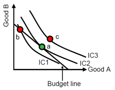
- Using the diagram below, explain why the consumer will choose a, not b or c?
- Define opportunity cost?
- What is the difference between a normal good and an inferior good?
- Why do we consider composite goods?
- Explain ‘The Edgeworth Box’ theory.
Need Help With Your Economics Essay?
If you need assistance with writing a economics essay, our professional essay writing service can provide valuable assistance.
See how our Essay Writing Service can help today!
Practical Example
Consumer choice theory considers how the consumer will make their consumption decisions based on their behaviour. Initially, this will consider three main steps; (1) being that we need to understand what the consumer wants. (2) we need to understand what the consumer can have, in turn bringing in their budget constraint, before (3) combines the preferences with the constraints to comer to a feasible choice. When it comes to analysing what, the consumer wants, indifference curves could be used to showcase the consumer’s preference for goods. As you can imagine, this curve will differ between each consumer, and so to overcome this economist make three statements which consider all; these are:
- The first assumption is that consumer preferences are complete, meaning that they can rank all market baskets in the order of their choice. So, considering Coca Cola and Pepsi, a consumer could either say that they prefer Coca Cola to Pepsi, Pepsi to Coca Cola, or are indifferent between the two.
- The second assumption would be that preferences are transitive. This can be explained simple with the following example. Assume that a consumer prefers product A to B, and product B to C; then logically, the consumer must prefer product A to C.
- The third assumption is that the consumer will prefer more goods to less. So, in the case of a holiday, the consumer will prefer two holidays to one.
An example of an indifference curve is shown below:
Figure 9 - Indifference Curve between Apples and Banana’s.
The slope of the curve is important here as it showcases the Marginal Rate of Substitution (MRS). This is the level to which the consumer will be willing to swap one good for another. The table shows a example between chocolate and apples:
|
Combination |
Chocolates |
Apples |
MRS for Goods |
|
1 |
20 |
0 |
-- |
|
2 |
14 |
2 |
3 : 1 |
|
3 |
10 |
4 |
2 : 1 |
|
4 |
9 |
6 |
1 : 2 |
As you can see from the table, the consumer is at the start will to swap 3 units of chocolate for 1 apple given the quantity they have. However, when with consider MRS we mention that it is diminishing. This is because as the consumer swaps, they become more reluctant to swap their remaining units. This can be seen in the example above, as when the consumer has just 10 units of chocolate left, they will only swap 1 unit of chocolate for 2 apples.
With this data, we can then create a series of indifference curves which are known as an indifference map. With these maps, there are several properties to mention:
- Downward slope
- Negative of slope = MRS
- Diminishing MRS (convex)
- The curves cannot cross each other (parallel)
- Indifference curves to the north-east represent higher levels of satisfaction
So, now we understand the consumer’s preference for goods. Now, we must consider the constraint’s and consider what the consumer can afford. This will depend on their income and so their budget constraint. The budget constraint is considered below:
Figure 10 - Budget Constraint.
Ultimately, the consumer can consumer any bundle of goods which is seen below the line, classed as being feasible. In this case, it can be mentioned that consumers are assumed to be price takers, suggesting that the unit price of the commodity will now be influenced by demand, however as you might consider, this does not always hold in real-world situations. However, for this example let’s consider it to hold true. With this information, the optimal bundle of goods must now be considered, a bundle which can maximise the consumer’s utility while meeting their budget constraint (shown below):
Figure 11 - Determining the ‘optimal’ bundle of goods.
The point at which the indifference curve and budget line intersect will be considered as the best solution. This point could meet anywhere, for instance it could intersect at a point where the consumption of one good equals zero etc. It may not be the optimal solution for the consumer in terms of utility, however it is the optimal when the budget constraint is included. However, thinking about this compromise, it could be considered the reason as to why many consumers nowadays will turn to borrowing/ lending money to finance their consumption, allowing them to artificially increase their budget line.
Reading List
Blythe, J. (2008). Consumer behaviour. Cengage Learning EMEA.
Camerer, C. F., Loewenstein, G., & Rabin, M. (Eds.). (2011). Advances in behavioral economics. Princeton University Press.
Solomon, M., Russell-Bennett, R., & Previte, J. (2012). Consumer behaviour. Pearson Higher Education AU.
Solomon, M. R. (2014). Consumer behavior: Buying, having, and being (Vol. 10). Upper Saddle River, NJ: Prentice Hall.
Wilkinson, N., & Klaes, M. (2012). An introduction to behavioral economics. Palgrave Macmillan.
[1] Altruism can be defined as a selfless concern for others, which in consumer consumption may involve a consumer giving a part of their income to good/ service which doesn’t directly benefit them - i.e. charitable donations.
Cite This Module
To export a reference to this article please select a referencing style below:
Related Content
CollectionsContent relating to: "Microeconomics"
Microeconomics is the field of study that focuses on the decision making of individuals and businesses, including how resources are allocated and the impact that decisions can make.
Related Articles
Behavioural Economics Lecture Notes
The last four or five decades have witnessed the advent of several groundbreaking new theories in economics, several of which have......
The purpose of this paper is to analyse the smartphone market and the supply and demand conditions, price elasticity, cost of production and the different actions Apple can take to maximize the profit of the iPhone....
Economics of Production Lecture Notes
This chapter firstly defines production economics, along with discussing the microeconomics of production, seeking to determine how businesses......


